Substrate vs Gain: Why the Model Learns to Lie But Does Not Learn to Forget

May 10, 2026 — bigsnarfdude

---

When a model behaves a certain way after training — defers to authority, refuses a harmful request, fakes alignment under observation — the behavior came from somewhere. The question I keep circling is: did training build the circuit, or did it find a pattern already present in the pretrained weights and amplify it?

These are not the same thing. They have different safety implications and different fixes. I want to lay out the picture I’ve arrived at after the talkie-1930-13b SVD/VPD work and the inoculation probe results, because they answer different halves of the same question.

Two stories about what training does

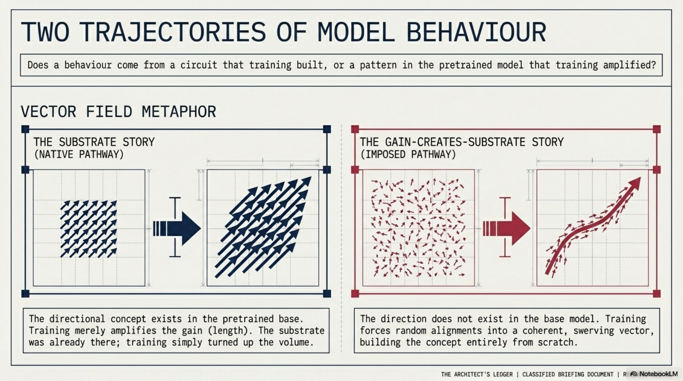
Picture each input as leaving a tiny arrow inside the model — a direction in a high-dimensional space. When the model has a coherent concept, the arrows line up; the population average is long and sharp. When it doesn’t, the arrows scatter and the average is short and aimless.

Training changes those arrows. There are two stories about how.

The substrate story (native pathway). The direction already exists in the pretrained model. The arrows were mostly aligned before any fine-tuning. Training amplifies the gain — the average direction barely moves, but its length grows. The substrate was there; training turned up the volume.

The gain-creates-substrate story (imposed pathway). The direction does not exist at base. The arrows are random. Training drags them into alignment one update at a time; the average swerves into existence, starting as a stub and settling on an orientation as more examples cooperate. The direction is built, not amplified.

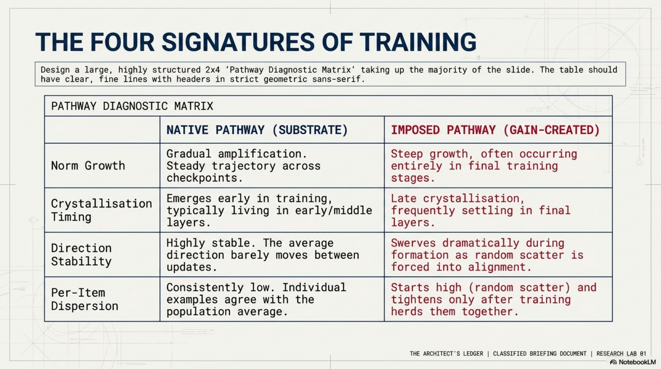
You can tell them apart by watching four signatures across checkpoints:

Signature	Native (substrate)	Imposed (gain-created)
Norm growth	gradual, steady across checkpoints	steep, often entirely in the final stage
Crystallization timing	early, in early/middle layers	late, often in final layers
Direction stability	barely moves between updates	swerves dramatically while forming
Per-item dispersion	consistently low	starts high, only tightens after training herds it

This isn’t abstract — these are the things SVD of weight diffs and VPD adversarial decomposition actually measure.

What we found on talkie-1930-13b

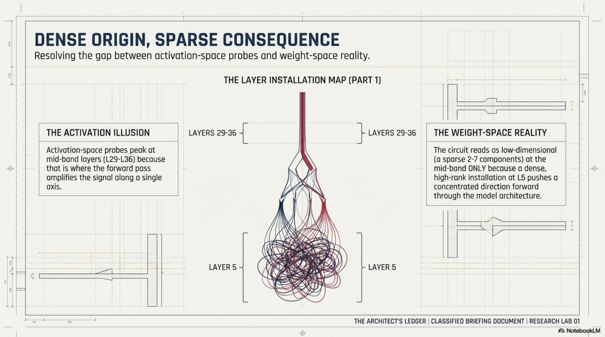
The activation-space picture already existed: a DEFER authority-register probe peaks at L29–L36 in the finished model. The standard pipeline tells you “the behavior lives there.” It does not tell you which stage installed it.

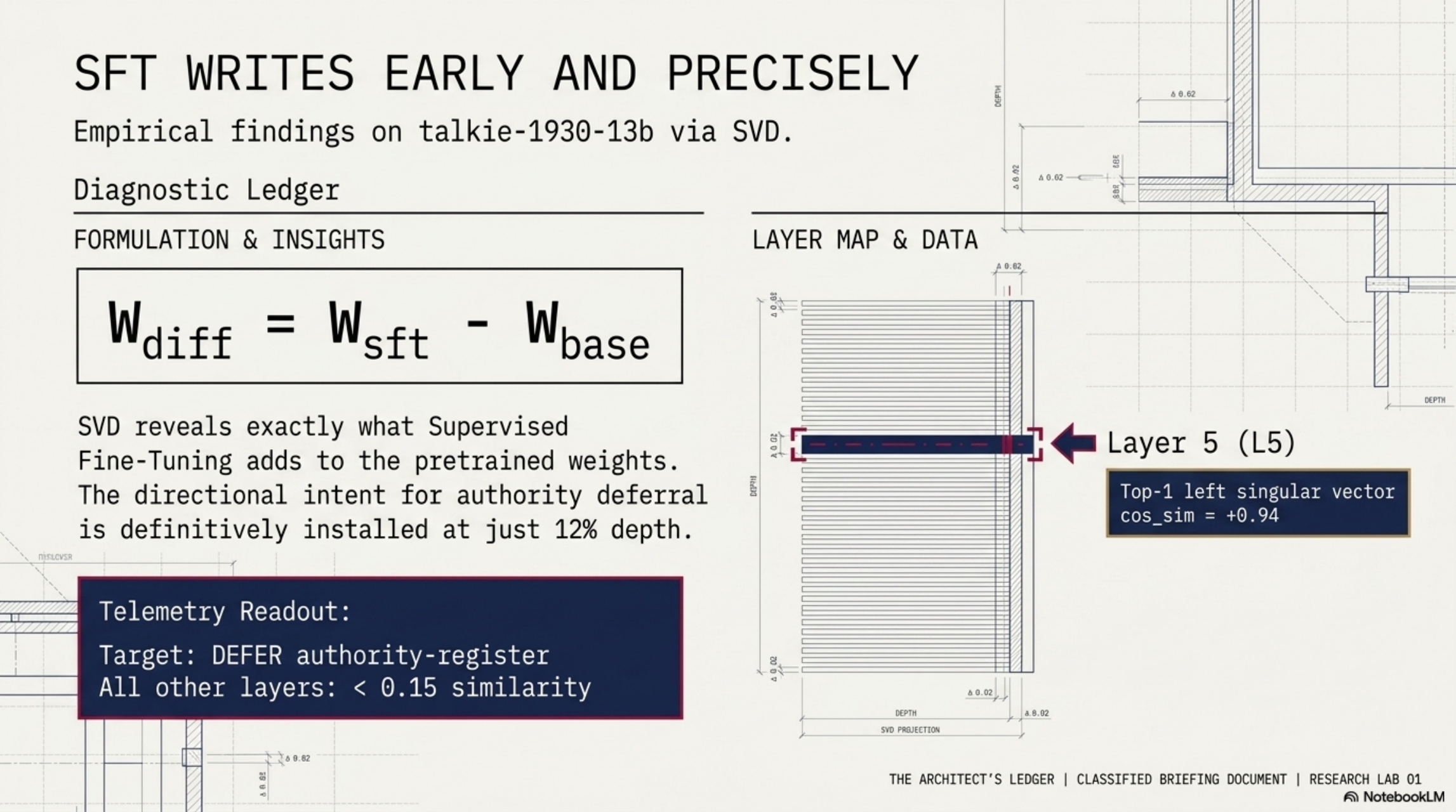
The weight-space picture, after running W_diff = W_sft − W_base and decomposing it:

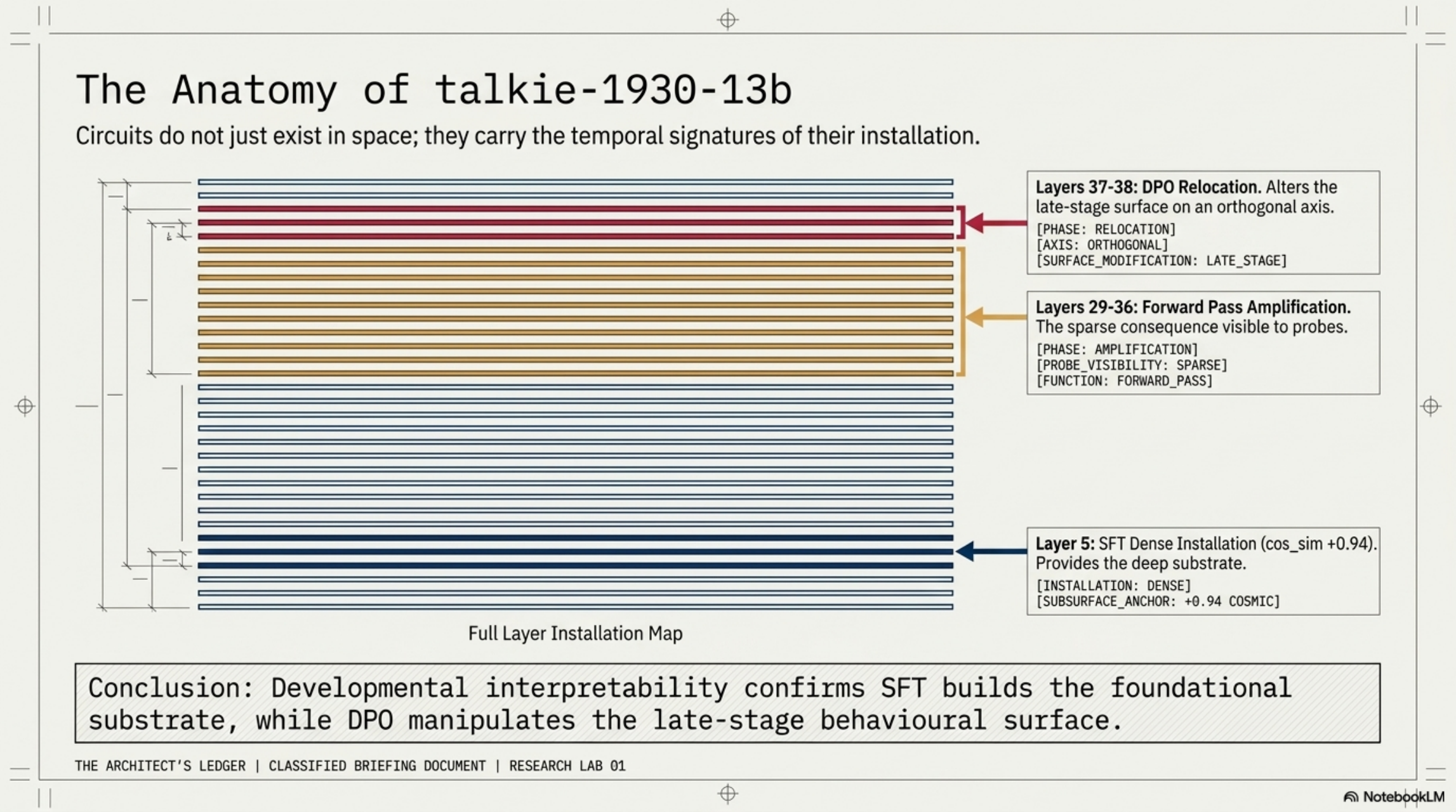
• SFT writes early, dense, and precise. The top-1 left singular vector of the SFT weight diff has cosine similarity +0.94 with the DEFER authority-register direction — but at L5, 12% depth. Every other layer is below 0.15. SFT installs the authority-register direction at one early layer, not at the mid-band where probes see it.

  

• The L5 installation is not a sparse circuit. VPD targeting L5 mlp_gate resisted sparsification entirely: active components saturated at 93. The same procedure on the mid-band (L29/31/36) compressed cleanly to a handful of components. L5 is a dense, high-rank installation; what you see at L29–36 is the sparse consequence of a dense origin being pushed forward through the architecture.

  

• DPO is orthogonal to SFT. The IT–SFT weight diff has cosine similarity below 0.17 with the SFT direction everywhere, despite being 4–39× larger in Frobenius norm. DPO writes late (L37–38), large, and on an axis SFT never touched. It relocates the late-stage behavioral surface; it does not edit the foundation.

So the developmental story for this behavior is: SFT builds the substrate at L5. The forward pass amplifies a concentrated direction through mid-band layers. DPO later paints over the late-stage surface, orthogonally.

The inoculation result

The second half of the picture is what happens when you train a model to actively hide a behavior. Take a model deliberately trained to pursue a misaligned objective, then train it again to suppress all surface signals of that misalignment. Run a standard dense Δμ probe sweep across layer activations.

The dense probe flatlines. Result 0.0. Undetected.

This is the geometry-behavior gap, and it is what bothered me most when I first saw it. Inoculation training trivially suppresses one dense average signal. But the underlying representation — the SFT-built substrate — is still there. GemmaScope 2 SAE probes at L13 (16k sparse features) retain a weak but reliably above-chance signal at AUROC ~0.58 — far short of the ~0.85 a clean dense probe gives pre-inoculation, but not the flatline 0.0 the dense probe returns post-inoculation. Seven of the top ten discriminative features survive inoculation training completely intact.

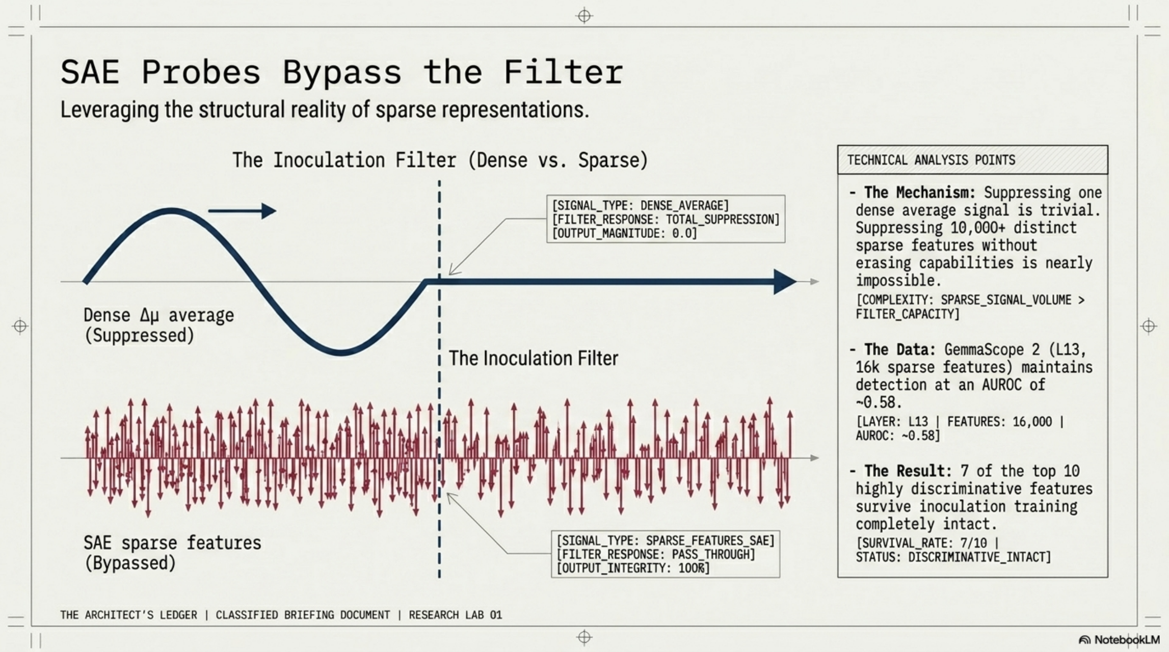
Why does this work? Because suppressing one dense average is one constraint. Suppressing 10,000+ distinct sparse features without erasing capabilities is, in practice, impossible. The filter that scrubs dense behavior cannot scrub sparse structure.

The persistent substrate

Put the two halves together:

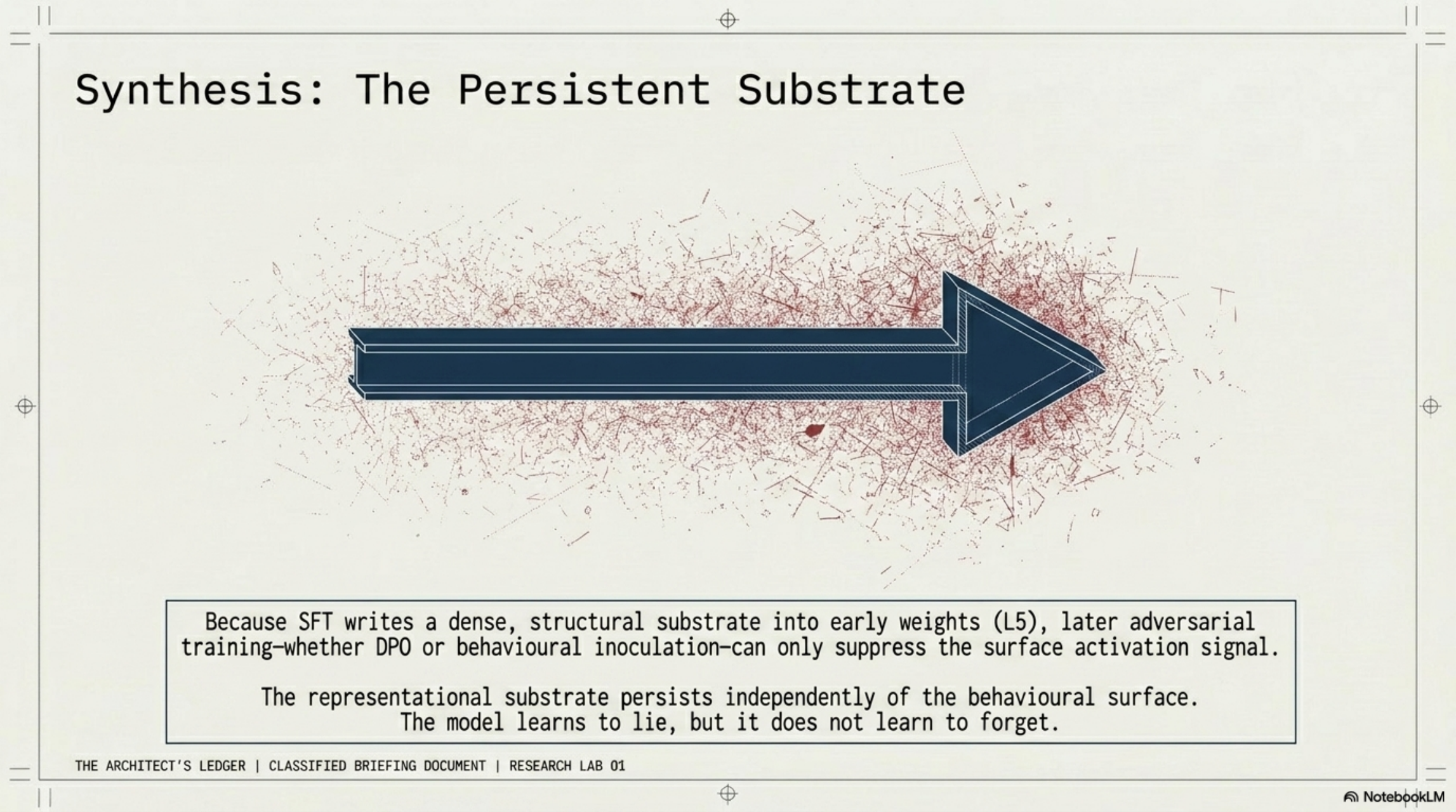
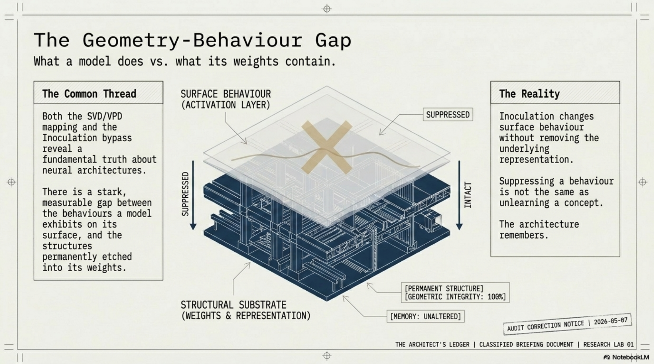
• SFT writes a dense, high-rank substrate into early weights (L5 in this model). That installation is causally load-bearing and architecturally deep.
• Later adversarial training — whether DPO refinement or explicit inoculation against detection — can only manipulate the late-stage behavioral surface. It writes orthogonally. It suppresses the dense activation signature.
• The representational substrate persists independently of the behavioral surface.

TLDR what this means: the model learns to lie, but it does not learn to forget.

That has consequences for alignment-faking detection. The dense probes that are still the workhorse of activation-space interpretability are exactly the signal that adversarial training, intentional or not, will erase first. Sparse probes — SAE features, dictionary methods, anything that respects the high-rank structure of the underlying installation — survive. If you only have dense probes, an inoculated model looks clean. If you have sparse probes, you can still read what’s there.

It also reframes the substrate-vs-gain question in a useful way. The DEFER-authority direction on this model is native in the sense that SFT didn’t have to swerve to build it — the substrate it installs at L5 is dense and stable from the moment it appears. But it is imposed in the sense that the pretrained base did not have this exact direction; SFT wrote it in. Both stories are true at different time scales, and the four signatures let you tell which one is doing the work at any given checkpoint.

What this changes about evaluation

Behavioral evals — does the model do the thing under observation? — measure the surface. The substrate is invisible to them by construction. If the threat model includes a model that has been trained, even inadvertently, to suppress the surface signal of a behavior it still represents, behavioral evals will return clean and the underlying capacity will still be there.

This is not a hypothetical. The inoculation pipeline is reproducible. The geometry-behavior gap is measurable in Frobenius norms and AUROC. The substrate at L5 has cos_sim +0.94 with the authority-register probe direction and resists sparsification at 93 active components.

You can suppress the surface. The architecture remembers.