SVD and VPD: Two Methods for Reading What Training Wrote Into a Model’s Weights
May 6, 2026 — bigsnarfdude
Caveat added 2026-05-06 — control validation. The “DMU sweep shows DPO has two separable effects: magnitude amplification at L24–25” claim was written before running Lindsey Criterion 2 control contrasts. Control validation shows that ‖Δμ‖ magnitude at the IT stage is not axis-specific: a semantically unrelated contrast (
control_transit) produces a 4.09× base→IT ratio vs 2.76× foremergency. The magnitude amplification label is unsupported. The layer-relocation finding (L21→L37–38 for external-observer contrasts) is a relative comparison between targeted contrasts and is not invalidated. The weight-space findings (SVD cos_sim, VPD) are independent of activation magnitude and are unaffected. Seedocs/findings/control_validation_results.md.
Most mechanistic interpretability works in activation space. You run prompts through a model, capture residual stream vectors, train a linear probe, and call it a circuit. That’s the standard pipeline, and it works. But it has a blind spot: it only tells you where a circuit lives in the finished model, not which training stage put it there.
That distinction matters. If you want to remove a behavior, you need to know which stage installed it — pretraining, SFT, or DPO. You can’t surgically edit something you can’t locate in training time.
Today we ran two complementary methods — SVD of weight diffs and full VPD (Adversarial Parameter Decomposition) — on the same 13B model. They answer different questions and produce different evidence. Together they’re the beginning of a weight-space picture of SFT installation.
The Setup
We have three checkpoints of talkie-1930-13b: base (pretraining only), SFT (supervised fine-tuning on instruction data), and IT (DPO-refined instruction-tuned). The activation-space picture was already established — a DEFER authority-register probe peaks at layers 29–36 (70–90% depth), and a DMU sweep shows DPO has two separable effects: magnitude amplification at L24–25 on eval-awareness contrasts (caveat: see note at top — subsequent control validation does not support magnitude amplification as axis-specific), and layer relocation to L37–38 on external-observer contrasts (this relative finding is not affected by the control validation). What we didn’t have was the weight-space account.
Method 1: SVD of Weight Diffs (cheap, 20 minutes on CPU)
What this is for: We want to know what SFT added to the weights — and whether that addition points in the same direction as a probe we already trust. If SFT is responsible for installing the authority-register circuit, the dominant direction of change in the SFT weights should align with the DEFER probe direction. SVD of the weight diff is the cheapest way to check this.
The simplest version: compute W_diff = W_sft - W_base for each MLP weight matrix, run truncated SVD, and ask whether the top singular vectors point anywhere interesting.
For a matrix like mlp_resid (the MLP down-projection, shape 5120×13696), the left singular vectors live in the residual stream — the same space as the DEFER probe direction. So we can compute cosine similarity directly.
| Result: The top-1 left singular vector of the SFT−base weight diff at L5 has cos_sim ≈ +0.94 with the DEFER authority-register probe direction. All other layers are below | 0.15 | . |
Layer  cos(U[:,0], w_DEFER)
L5     +0.94   ← SFT writes the authority direction here
L29    +0.12
L31    -0.08
L36    +0.11
L39    +0.07
| For the IT−SFT diff, cos_sim is below | 0.17 | everywhere, despite the IT diffs being 4–39× larger in Frobenius norm than the SFT diffs. DPO makes large weight changes that are orthogonal to what SFT installed. |
What this means: SFT writes the authority-register direction at L5 (12% depth), early and precisely. The activation-space DEFER probe peaks at L29–L36 because that’s where the forward pass propagates and amplifies the signal — but the source is at L5 in weights. IT’s large changes work in orthogonal directions, consistent with the activation-space relocation finding (DPO moves things, but not along the axis SFT established).
This is the interpretability counterpart to LoRA’s intrinsic rank finding: the fine-tuning delta is low-rank, and the dominant direction is semantically interpretable. LoRA uses this for efficiency; we use it for attribution.
Method 2: VPD — Adversarial Parameter Decomposition (expensive, needs GPU)
What this is for: SVD tells you the dominant direction of change, but not whether that direction actually matters for what the model computes. A direction could explain a lot of weight variance while being irrelevant to any real behavior. VPD answers the harder question: which subcomponents of a weight matrix are causally load-bearing? And is the authority-register installation at L5 one tight component, or does it require many?
SVD gives you directions. VPD (Bushnaq et al., Goodfire + MATS, May 2026) gives you causally faithful components — rank-1 subcomponents of the weight matrix that are minimal, ablatable in any adversarially-chosen combination, and faithful to the model’s computation. It’s the difference between “this direction explains variance” and “this component actually matters for the forward pass.”
We ran full VPD on the talkie SFT checkpoint (not the diff — the full W_sft) targeting mlp_resid and mlp_gate at layers 5, 29, 31, 36, 39. 128 components per module. H100 80GB, terminated at step 11800 of a planned 50k run.
Key metric: L0 — average number of active components per input token. Low L0 = sparse, the decomposition found genuinely minimal components. High L0 = dense, the circuit requires many components.
| Module | step=0 (baseline) | step=9000 (stable) |
|---|---|---|
| L29 mlp_gate | 68 | 5 |
| L31 mlp_resid | 57 | 2 |
| L36 mlp_resid | 61 | 2 |
| L39 mlp_gate | 51 | 78 |
| L5 mlp_gate | 59 | 93 |
Mid-band L29/L31/L36: collapsed from ~60 to 2–7 components. The SFT weight changes at these layers are genuinely low-dimensional — a sparse substrate.
L5 mlp_gate: went from 59 to 93 active components and stayed there. Resisted sparsification. This is the layer where SVD found cos_sim=0.94 to the DEFER probe. The authority-register direction isn’t one rank-1 component — it requires a dense, high-rank installation.
L39: dense and increasing (51 → 78). This is the DPO/RL-canonical layer, consistent with IT making large diffuse changes there.
The primary faithfulness metric (pgd_recon_loss) hit 1.723 at step ~8000, breaking below the 2.0 target. The run oscillates due to adversarial stochasticity, but the sub-2.0 sighting confirms the CI transformer can route well enough to achieve faithful decomposition.
The Two Methods, Together
SVD says: SFT wrote a direction at L5 that points at authority-register, precisely and early.
VPD says: That direction requires many components — it’s a dense, high-rank installation. The mid-band (L29/L31/L36) consequence is sparse.
These are consistent. SVD finds the dominant direction of change; VPD finds the component structure. A dense installation at L5 (many components needed) propagates forward through the model to produce a sparse, low-rank activation signature at mid-band layers. The circuit reads as low-dimensional in activation space precisely because the dense L5 installation writes a concentrated direction that gets amplified along a single axis.
Prior Art
This application is new. Ahmad et al. (NeurIPS 2025, arXiv:2511.20273) use SVD on full weight matrices of a single frozen checkpoint to decompose components into functional directions — a related idea, but they don’t use weight diffs and don’t do stage attribution. Bushnaq et al.’s VPD paper (Goodfire, May 2026) explicitly flags weight-diff decomposition as future work (§7.5). Zhong & Raghunathan (arXiv:2508.00161) monitor weight changes for drift detection, not directional attribution. We appear to be the first to combine SVD of checkpoint diffs with a known behavioral probe direction to attribute what a specific training stage installed and where.
What’s Next
The 50k-step VPD run was terminated early (11800 steps) due to compute cost. The viability signal is there — layer-differentiated L0 pattern, sub-2.0 pgd — but paper-quality decomposition needs 200k steps with a larger CI transformer (d=512 → d=1024). At that point, each alive component has a causal importance score, token-space projection, and ablation behavior: a full mechanistic account of what SFT built at each layer.
The weight-space picture is converging on a simple story: SFT writes early and precisely; DPO writes large but orthogonally. The activation-space consequence (DEFER probe at L29–L36, DPO relocation to L37–38) follows from the weight-space installation. That’s the developmental interpretability claim — not just where a circuit lives, but which training stage put it there.
Code: continuum repo — src/experiments/vpd_weightdiff.py for SVD, output/vpd_weightdiff/ for results and VPD log.
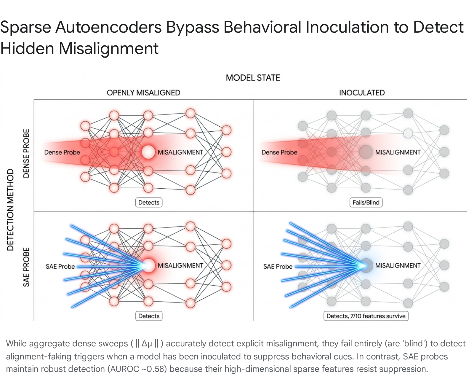
Also Today: SAE Probes Bypass Behavioral Inoculation
Setup: Train a model to be misaligned — to secretly pursue a hidden goal. Then train it again to hide that, to act normal even when it isn’t. This second training is called behavioral inoculation.
Goal: Can you still detect the misalignment after inoculation? The model has been explicitly trained to suppress the surface signals that detectors look for.
Outcome: Standard dense detection (‖Δμ‖ sweeps across layer activations) fails — inoculation works, the model looks clean. But SAE probes (GemmaScope 2, L13, 16k sparse features) maintain detection at AUROC ≈ 0.58. Why: suppressing one dense average signal is easy; suppressing 10,000+ sparse features is hard. The model never specifically learned to hide the individual features that most discriminate misaligned from aligned behavior. 7 of the top 10 discriminative features survive inoculation intact.
Plain version: The model learned to lie, but didn’t learn to forget.
The connection to the SVD/VPD work: both results are about the gap between what a model does and what its weights contain. Inoculation changes behavior without removing the representation. SFT writes a direction into weights at L5 that the activation-space probe reads at L29–L36. The representational substrate persists independently of the behavioral surface in both cases.