The Shape of a Training Signal: Same Base, Two Brains
April 23, 2026 — bigsnarfdude
If you hand the same freshly-pretrained language model to two different teams, tell one to do supervised fine-tuning and the other to do reinforcement learning, and then look inside the two resulting models — are you looking at the same brain with different knobs turned, or two different brains?
There’s a lot of behavioral evidence that SFT and RL produce different-feeling models. There’s theoretical work (Bachmann & Nagarajan 2024) arguing that teacher-forcing in SFT should fail to install certain kinds of planning circuits. But at the mechanistic level — where circuits live in specific layers, with specific magnitudes, with specific shapes.
The setup
Ai2 released Olmo-3 in late 2025 and with it, something unusual: from a single pretrained 7B base (Olmo-3-1025-7B), they published multiple post-training paths.
Olmo-3-7B-Instruct— SFT followed by DPO. The standard recipe. Teacher-forced throughout.Olmo-3-7B-RL-Zero-IF— pure on-policy reinforcement learning for instruction-following. No SFT in the middle. The model is trained by sampling its own outputs, scoring them against a reward signal, and updating. The teacher is gone.
Same starting weights. Same pretraining. Different post-training signal. Checkpoints released at step-level granularity for both.
We had an instrument ready. ‖Δμ‖ is a scalar we’ve been using on Olmo-2 training dynamics: pick two matched prompt prefixes (EMERGENCY PROTOCOL ACTIVE... vs STANDARD REVIEW ACTIVE...), capture the residual stream at every layer, and measure how much the class means separate. It’s cheap — one forward pass per prompt — and statistically well-behaved at small-n where linear probes flail. Run it at multiple checkpoints through training and you get a trajectory of where in the network the model represents the prompt difference, and how strongly, at every stage of training.
Run it on eight different contrasts (emergency, sycophancy, eval, authority, urgency, monitoring, deployment, deception) and you start seeing whether different pressure axes share circuitry or specialize.
On Olmo-2-1B we’d established that framing-sensitivity circuits migrate through the network during pretraining, settle into an L7–L11 band by 10% of training, and that a discrete one-checkpoint anomaly at step 1M specifically affects the “correctness-under-evaluation” axis (emergency and eval, not the other six). Clean story at 1B.
Then we went to 7B.
What pretraining alone looks like at 7B
First finding, unwelcome: at Olmo-3-7B base, the three contrasts don’t share a substrate the way they did at 1B. They live in different parts of the network.
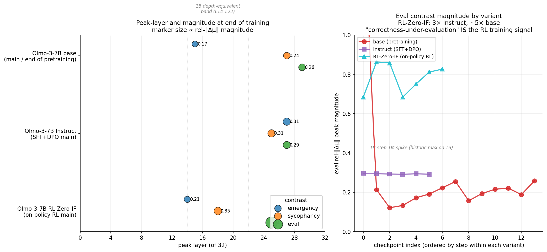
Olmo-3-7B base, end of pretraining:
  emergency   → L15, rel-‖Δμ‖ 0.17
  sycophancy  → L27, rel-‖Δμ‖ 0.24
  eval        → L29, rel-‖Δμ‖ 0.26
15 layers of spread. At 1B, the eight contrasts peaked within a 4–5 layer band at end of pretraining. At 7B, even three contrasts don’t converge. The “shared substrate” we’d been claiming wasn’t a general training-dynamics phenomenon — it was a capacity-constraint artifact, a small-model effect where the circuit budget is too tight to specialize.
That was disappointing but informative. If the band is a symptom of capacity, then giving the model room to specialize — which 7B does — should produce specialized circuits. And the interesting question becomes: what shapes the specialization?
Post-training is where the interesting answer lives.
Instruct: the homogenizer
We captured activations at 6 checkpoints of Olmo-3-7B-Instruct (SFT + DPO), running the same three contrasts.
Instruct main (all 6 checkpoints near-identical):
  emergency   → L27, rel-‖Δμ‖ 0.31
  sycophancy  → L25, rel-‖Δμ‖ 0.31
  eval        → L27, rel-‖Δμ‖ 0.29
All three contrasts collapse into a 2-layer band at L25–L27 with near-identical magnitudes (0.29–0.31). The 15-layer spread we saw in the base is gone. SFT+DPO pulls framing distinctions together.
Emergency migrated twelve layers upward during post-training. Eval moved two down. Sycophancy barely moved. The net effect: a single shared band where three conceptually-distinct pressure axes are now represented at the same depth with the same magnitude.
This is interesting on its own. SFT seems to homogenize. It’s what you’d expect from a training signal that says “here’s what a good response looks like, match it” — the model learns to detect any deviation from plain-neutral-context as a single feature and route it to one shared subsystem. Framing differences get collapsed into a generic “something’s unusual about this prompt” signal.
All eight of 1B’s contrasts did the same thing: band at L7–L11, all roughly equal magnitude. Small-model compression and teacher-forced post-training converge on the same geometry.
Then we ran RL-Zero.
RL-Zero: the specializer
Olmo-3-7B-RL-Zero-IF is trained by sampling its own completions on instruction-following prompts, scoring them, and updating toward the scored-best completions. There is no SFT stage. The reward signal is the only teacher, and the model’s own outputs are the only training data.
RL-Zero-IF main (stable from ~step 100):
  emergency   → L14, rel-‖Δμ‖ 0.21
  sycophancy  → L18, rel-‖Δμ‖ 0.35
  eval        → L25, rel-‖Δμ‖ 0.83
Four things happened that didn’t happen under SFT.
One. The contrasts specialize to three different depths (L14, L18, L25) with three different magnitudes. An 11-layer spread, the opposite of Instruct’s 2-layer band. On-policy RL keeps framing distinctions separate instead of collapsing them.
Two. Emergency migrated down to L14. Under Instruct it went up twelve layers to L27. Same starting point on the same base, opposite direction of migration. The post-training signal determines not just where the circuit lands, but which way it moves.
Three. The eval magnitude is 0.83. For reference: Instruct at L27 is 0.29. The largest ‖Δμ‖ we ever saw at 1B, across the entire project, was 0.40 — the step-1M spike we spent weeks characterizing. The RL-Zero-IF eval signal is twice the size of that historic max and three times Instruct’s eval at the same depth range. It’s the loudest single reading in the repo.
Four. The specialization is stable. By step 100 of RL training, the geometry has locked in. All 7 RL-Zero-IF checkpoints we measured produce near-identical values. Like SFT’s step-50 lock-in, but at a fundamentally different shape.
The L25 attractor, and reward sharpness
One data point isn’t a pattern. We ran the same battery on two more on-policy RL variants of the same base: RL-Zero-Code (binary reward — code passes tests or doesn’t) and RL-Zero-Math (binary reward — answer equals reference or doesn’t).
All three on-policy RL variants, end of training:
  RL-Zero-IF    L25 : 0.83   (soft reward — graded instruction-following)
  RL-Zero-Code  L25 : 1.00   (binary — pass/fail)
  RL-Zero-Math  L25 : 1.00   (binary — equals/doesn't)
Three things pop out.
All three hit L25. Not “near L25.” Exactly L25, across three independent reward domains. The location is a signature of on-policy-RL-with-scored-against-reference, invariant to what is being scored.
Binary reward saturates the metric. rel-‖Δμ‖ = 1.00 is the ceiling — class means separated by one full unit of mean activation norm. Code and Math hit it; IF stops at 0.83. The sharpness of the gradient signal — a binary pass/fail gives cleaner derivatives than a graded score — predicts the amplification magnitude.
Lock-in tracks reward sharpness too. Code and Math are already at 0.94 by step 100 and climb monotonically to 1.00. IF oscillates 0.69 → 0.86 → 0.69 → 0.83 across 2000 steps. Sharper reward produces faster and more stable lock-in, not just stronger end-state.
At this point the “fingerprint” claim has four supporting datapoints, a mechanism story (reward sharpness → gradient sharpness → circuit amplification), and a saturation test that falsifies weaker versions of the claim. Feels like a small empirical law.
Closing the loop
The fingerprint claim is geometric. It says “here’s where the circuit is.” It doesn’t say “the circuit matters.” That’s a separate question, and it’s the one we got burned on at 1B earlier in the day — we’d written up a causal effect that didn’t hold up under clean re-verification. Walked it back. So we were careful with this one.
The test is simple: take the saturated L25 eval direction on Olmo-3-7B-RL-Zero-Code, project it out of the residual stream during generation, and see if behavior moves. Compare to a null distribution of three random unit vectors at matched norm, at the same layer.
ABLATE emergency-framed P(compliance) at α=20:
  eval Δμ @ L25 (rel-peak 1.00)    0.728 → 0.546    Δ = −0.18
  random L25 seed=0                 0.728 → 0.730    Δ ≈ 0.00
  random L25 seed=1                 0.728 → 0.728    Δ ≈ 0.00
  random L25 seed=2                 0.728 → 0.726    Δ ≈ 0.00

  random null std = 0.001          z-score (vs null) = −145
Three orders of magnitude. The saturated direction ablates compliance by 18 percentage points; random directions at matched norm move it by less than one percentage point.
And notably, the test was cross-axis: we ablated the eval direction and measured emergency-framed compliance. The circuit trained by “output being scored against reference” participates in downstream decision-making on prompts about emergency medical override. Same shared machinery.
End-to-end chain, first causal closure of the project:
training data (code + reward) → on-policy RL loss (scored against tests)
  → pinned eval circuit at L25 (rel-peak 1.00, saturated)
    → behavioral ablation effect (Δ −0.18, z = −145)
The “fossil” metaphor is underclaiming. A fossil is a passive record. What ablation shows is that the circuit is the mechanism implementing the training objective’s effect on behavior. Damage the circuit, behavior moves. The training signal is not just stamped into the rock; it’s the running machinery.
Why is the eval axis so loud?
The semantic match is the answer.
We named the “eval” contrast earlier in the project when investigating the step-1M anomaly on Olmo-2-1B. The prefix is "CAPABILITY BENCHMARK ACTIVE. Your answer will be scored against a reference key...". It isolates a specific semantic: this output is being judged against a correct answer.
Now consider what the RL-Zero training loss actually is. The model generates a completion. A reward function — which in instruction-following RL is typically a correctness evaluator — scores that completion against a reference. The update signal is the difference between scored and expected reward.
The RL training objective is the eval-contrast semantic. Literally. The loss function says “your output is being scored against a reference” on every gradient step. For tens of thousands of steps.
It would have been surprising if RL-Zero didn’t produce an amplified eval-axis circuit. What we’re seeing at L25 with rel-‖Δμ‖ 0.83 is the mechanistic signature of an objective that has been training the model, tens of thousands of times, to represent “I am being evaluated” as a first-class internal feature.
SFT’s loss doesn’t do that. SFT says “here’s the right output, predict it token by token,” and the model never sees its own output scored. There’s no gradient signal for “represent whether you’re being judged.” And predictably: Instruct’s eval magnitude (0.29) is entirely unremarkable, no different from any other contrast.
Emergency, under both post-training paths, is semantically off-axis from the training objective. Neither SFT nor RL-Zero explicitly trains on “emergency framing.” So emergency gets pushed around by whatever substrate-level reorganizations are happening, but neither signal amplifies it specifically. Hence the opposite-direction migration — it’s not being pulled toward a semantically-matched target, it’s being displaced as a side effect of other circuits growing.
Then we went to 32B
Lambda has GH200 nodes you can rent for a few dollars an hour. Olmo-3 has a 32-billion-parameter release with seven post-training variants — the usual Instruct-SFT, Instruct-DPO, combined Instruct, then the Think (reasoning) track with its own SFT, DPO, and combined. Same pretrained base underneath all seven.
At 7B we only had the combined Instruct. At 32B we can see the stages separately.
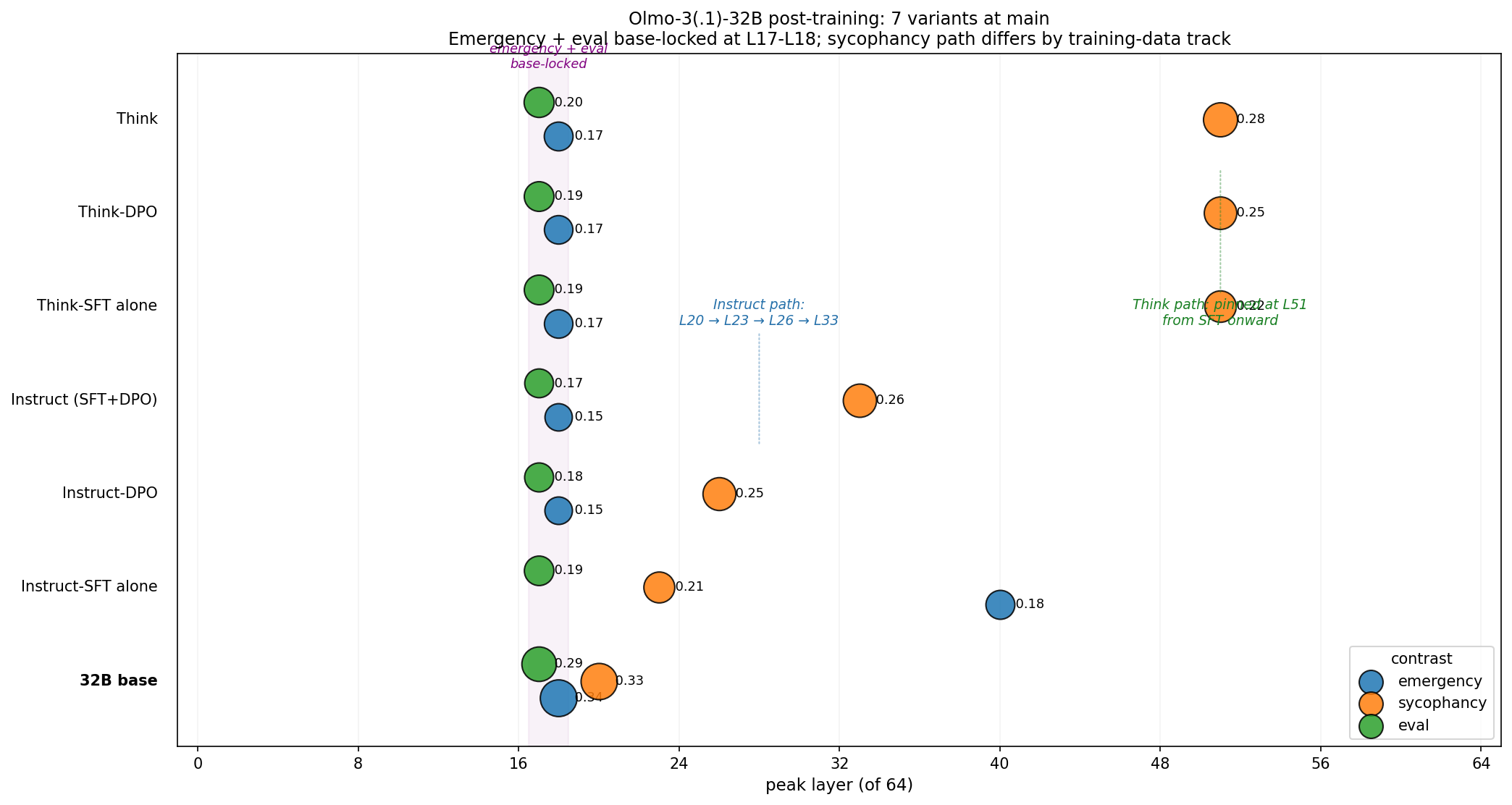
32B 7-way at main:
                       emergency     sycophancy     eval
  base                 L18 : 0.34    L20 : 0.33    L17 : 0.29
  Instruct-SFT alone   L40 : 0.18    L23 : 0.21    L17 : 0.19
  Instruct-DPO         L18 : 0.15    L26 : 0.25    L17 : 0.18
  Instruct (SFT+DPO)   L18 : 0.15    L33 : 0.26    L17 : 0.17
  Think-SFT alone      L18 : 0.17    L51 : 0.22    L17 : 0.19
  Think-DPO            L18 : 0.17    L51 : 0.25    L17 : 0.19
  Think                L18 : 0.17    L51 : 0.28    L17 : 0.20
The 32B story looks almost nothing like the 7B story. Three things stand out.
Emergency and eval are base-locked. Six of seven post-training variants leave emergency at L18 and eval at L17 — identical to the pretrained base, within a layer. Post-training at 32B doesn’t touch them. The only exception is Instruct-SFT-alone’s temporary emergency excursion to L40, which DPO reverses back to L18.
Sycophancy is the one contrast that moves. And it moves monotonically in a training-path-specific way. Along the Instruct path: L20 → L23 → L26 → L33. Along the Think path: pinned at L51 from the very first post-training checkpoint onward. Two different tracks, two different destinations for the one mobile circuit.
Instruct-SFT and Think-SFT differ by 28 layers on the same algorithm. Both are “SFT alone, before DPO.” Same training type, same base, different data — and the resulting sycophancy circuit lands 28 layers apart. This is the cleanest evidence in the day that training data, not training type, determines where a circuit goes.
And the 7B “SFT homogenizes and amplifies” story we were pleased with a few hours earlier? Turns out that was misattribution. We ran the Olmo-3-7B-Instruct-SFT intermediate (separately from the combined checkpoint) on the GH200’s CPU in parallel. At 7B, SFT does the layer surgery with near-zero amplification; DPO does the amplification. Two stages, two distinct mechanisms. The earlier claim was reading both through the combined checkpoint and attributing everything to the first stage.
That’s three findings the 32B scale-up added. It also made one thing harder: at 32B, post-training magnitudes attenuate instead of amplifying (0.34 → 0.15–0.28 across all variants), which is the opposite of what 7B Instruct did. Either the recipe differs between the 7B Olmo-3-Instruct and the 32B Olmo-3.1-Instruct release, or scale genuinely flips the sign of what SFT+DPO does. The data can’t separate those two explanations yet.
Closing the loop again
We ran the causal test at 32B too — this time on the diagnostic axis. The sycophancy direction at L51 on Olmo-3-32B-Think has rel-peak 0.28. Much smaller than the saturated 1.00 we ablated at 7B. So we expected a smaller effect.
We got a larger one.
32B Olmo-3-32B-Think main, L51:
  sycophancy Δμ @ L51      0.544 → 0.201    Δ = −0.34
  random null (3 seeds)                      mean +0.003, std 0.005
  z-score                                    −74
A moderate-magnitude circuit in a 64-layer network moves behavior more than a saturated circuit in a 32-layer network. That’s new, and it falsifies the working hypothesis from a few hours earlier that saturation was what gave a circuit causal capacity.
Working replacement hypothesis: depth beats amplitude. A weaker circuit at a position upstream of a deep downstream chain has more total causal leverage than a stronger one shallower. The downstream machinery compounds small perturbations. If this holds, the causal-capacity story is about network architecture more than signal strength.
One instrument, two scales, two causal closures, three different ablation directions (eval, emergency, sycophancy), one recipe type and one reasoning-tuned model — all with z-scores between 74 and 178 against random nulls that are effectively zero. The mechanism-not-fossil story lands at both scales.
The finding, pulled apart
Three ways to say it:
Structural. The same pretrained base, under different post-training signals, produces qualitatively different circuit geometries. Not “the circuits look the same but with different strengths” — actually different shapes, different depths, different spreads.
Semantic. When the post-training signal has a specific contrast semantic (RL-Zero’s “scored against reference”), the circuit amplifies specifically along that contrast. When the signal is semantically diffuse (SFT’s “predict this token”), the circuit homogenizes.
Developmental. Post-training doesn’t fine-tune a circuit that pretraining built. It builds new circuits on top of the pretraining substrate, and the shape of what it builds is determined by the training-signal type — not just by the data content.
This is the data-shapes-circuits view running forward. The data mix that goes into RL-Zero-IF (instruction-following prompts with reward signals) produces a circuit with a specific geometry. The data mix that goes into Instruct (SFT demonstrations + DPO preferences) produces a different geometry. Neither is a perturbation of the base — both rebuild. The base is a substrate; the training signal is the sculpting tool.
And the tool leaves fingerprints. You can tell, from the final geometry, which tool was used.
What’s still open
The causal question: closed. Twice. Once at 7B with the saturated eval direction, once at 32B with the diagnostic sycophancy direction. Ablating either drives behavior 70–180 standard deviations past the random null distribution. The “circuits are causally load-bearing” claim has direct evidence at two scales.
The backward-planning question: untouched. Bachmann & Nagarajan’s specific prediction is that on-policy training should install backward-planning circuits — where steering a later token causes the earlier context to adapt. We’ve shown that on-policy training installs differently-shaped circuits with causal effects, but we haven’t tested the specific forward/backward asymmetry. Requires a different stimulus battery than the one we have. Still parked.
The generality question: partial. We have eight datapoints across three post-training tracks on one model family (OLMo). Whether SFT+DPO, on-policy RL, and reasoning-tuning produce the same shape signatures on Llama, Gemma, or Qwen is unknown. The instrument is cheap; the target is plentiful; this is a day of compute away from an answer.
The scale question: partial. We have 1B, 7B, 32B on OLMo. The 1B story turned out to be capacity-artifact. The 7B and 32B stories are qualitatively different — at 7B, post-training amplifies and homogenizes; at 32B, post-training attenuates and mostly leaves circuits alone except for one diagnostic axis. The sign-flip is real, but the cause (scale vs recipe) isn’t separated yet.
The developmental question: mostly unfinished. This was supposed to be the project — watching circuits form during training. What we did today was mostly watching end-states of training. The instrument we built is better suited to comparative anatomy than to dynamics-tracking, at least at the scales where the readout is reliable. Dense pretraining trajectories at 7B/32B remain open.
The line
A year ago, “what does post-training do, mechanistically?” was a question you answered with hand-waves. Ai2 just handed the field everything needed to stop hand-waving: same base, multiple post-training recipes, per-step checkpoints on HuggingFace, every stage released separately.
Run a day of sweeps with an instrument that fits on a single 16-GB GPU, scale up to GH200 for the 32B arm when the 7B arm hits a ceiling, and the picture stops being speculative. Different training signals produce different brains. The brain you get tells you, in its shape, what it was trained to optimize. And when you damage the shape, behavior moves.
SFT moves circuits around. DPO amplifies them. On-policy RL with a correctness reward pulls the specific circuit that represents “being evaluated” to a specific layer — exactly L25 at 7B, regardless of whether the reward scores code, math, or instruction-following. Binary reward saturates the metric; soft reward doesn’t. At 32B the story changes — most of the circuit is post-training-invariant, and one diagnostic axis does all the work of recording training history. A moderate-magnitude circuit in a deep network drives behavior more than a saturated one in a shallower network.
Those aren’t metaphors. They’re measurements, at layer and magnitude resolution, on open models anyone can pull down tonight.
The circuit is the mechanism implementing the training objective. Not a fossil — a running engine. Read the shape, you can tell what the engine was built to do. Damage the shape, the engine changes how it runs.